New features in GS-Calc 20.3:
- Conditional cell formatting - the setFormatIf(reference, action, if_condition, format_true, format_false) formula
Formats a given cell or a range of cells. The numeric action parameter specifies which formatting attributes to set or clear (restore defaults).
Usually, it’s convenient to keep all the formatting functions in a separate worksheet. A single cell selection/value can control the appearances of other worksheets.
The function can be applied both to existing cells and empty regions without any previous formatting (and in this scenario the 1st update can be slightly slower).
There are no limitations for the number or complexity concerning this function. You can use millions of conditionally formatted cells or regions same as any other formulas and nested IFs.
If the reference argument specifies entire columns or rows, the formatting action will be applied respectively to column and row styles. The formatting layers are as follows: a table style < column styles < row styles < cell styles (and optionally colors defined in custom style patterns). Cell styles overwrite all other styles.
The format_true and format_false parameters be -1 to restore the default cell state for a given attribute or the following:
1 - numeric style (style index relative to the toolbar style list or the name)
2 - custom style pattern (custom style pattern like $#,##0.00)
3 - font size (4 to 256)
4 - font name (string)
6 - bold font (0 | 1)
7 - italic font (0 | 1)
8 - underline font (0 | 1)
9 - strikeout font (0 | 1)
11 - font color (RGB numeric value or a RGB string like “#FFEE00” or color name like “green”)
14 - horizontal alignment (0 - left, 1 - center, 2 - right)
15 - vertical alignment (0 - top, 1 - center, 2 - bottom)
16 - wrap text (0 | 1)
17 - horizontal indent (a number of pixels 0 to 64)
18 - vertical indent (a number of pixels 0 to 64)
19 - text rotation (a value in degrees between -180 to 180)
20 - cell borders (a string “position width style color” like “bottom 1px solid blue” or “all 1pt dotted #FF0000” or “dotted red”)
21 - borders around selection (a string “width style color” like “1px solid blue” or “thin solid #FF0000” or “dotted red”)
22 - cell background color (RGB numeric value or a RGB string like “#FFEE00” or color name like “green”)
25 - don’t print / print cells (0 | 1)
26 - hyperlink (0 | 1)
27 - cell with filters used by the filter() formula (0 | 1)
28 - cell with image lists (identified by built-in names, like “star start star-half”) (0 | 1)
29 - area in-cell chart (with the data series in cells pointed by the cell alignment, e.g. to the left) (0 | 1)
30 - column in-cell chart (0 | 1)
31 - bar in-cell chart (0 | 1)
32 - apply all 1-31 attributes at once as a named custom style (strings specified for custom styles in the “Format > Custom Cell Styles” dialog box
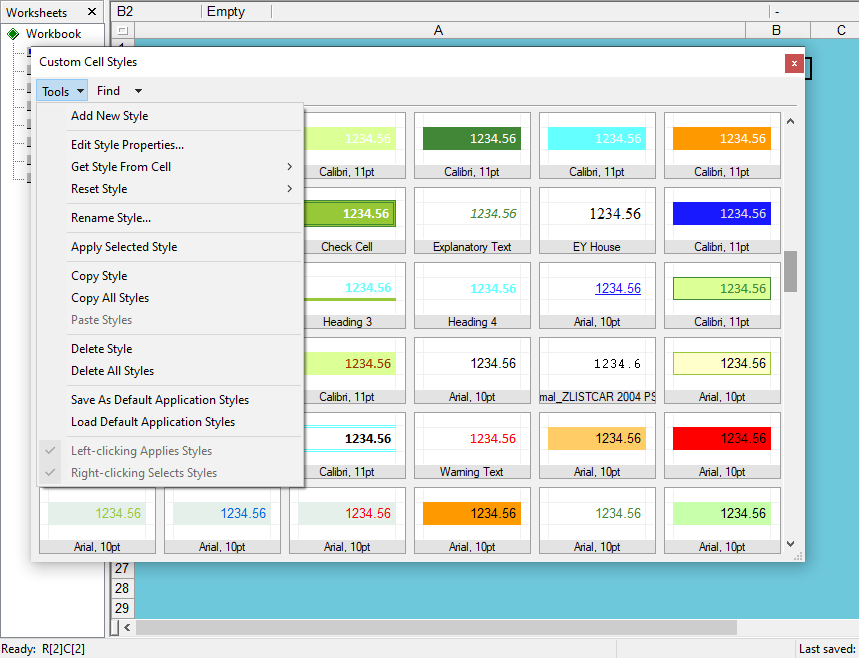
The 32nd action type sets all possible cell formatting/style attributes at once. Custom cell styles are added to a workbook with the Format > Custom Cell Styles dialog box and are saved in a workbook. Custom cell styles in a workbook can be saved to or loaded from a global GS-Calc cache using the Save As Default App Styles and Load Default App Styles commands in the Custom Cell Styles dialog box.
For the action = 20:
- The position attribute can be a space-separated list of the following names:
top
left
bottom
right
diag-left
diag-right- The width attribute can be:
- one of the names “thin”, “medium”, “thick”
- numeric values with suffixes indicating pixels (px), points (pt), inches (in), mm, cm or picas (pc)
- The style attribute can be:
solid
dotted
dash
long-dash
dot-dash
dot-dot-dash
wave
double - The color attribute can a numeric RGB value, a string representing the RGB triple e.g. “#FF0000” (which is red) or one of the predefined color names:
black
maroon
green
olive
navy
purple
teal
gray
silver
red
lime
yellow
blue
fuchsia
aqua
white
- The style attribute can be:
The function returns the evaluated value of the if_condition parameter.
The “Custom Cell Styles” dialog box:

https://citadel5.com/help/gscalc/custom-style2.png
The “Custom Cell Styles” dialog box and options:
https://citadel5.com/help/gscalc/custom-style3.png
Examples:
setFormatIf(c120, 11, c120 > 0, “green”, “red”)
setFormatIf(c:e, 11, c120 > 0, “green”, “red”)
setFormatIf(10:20, 11, c120 > 0, “green”, “red”)
setFormatIf(c120, 20, c120 > 0, “all 2px solid green”, “diag-left diag-right red”)
setFormatIf(d100:d999, 1, c1=“use format”, “currency”, 0)
setFormatIf(d99, 20, a1, “bottom 2px dotted green”, -1)
setFormatIf(d99, 32, a10 > 10, “my-style-1”, “my-style-2”)
- The “Update Selection (Alt+F9)” command has been added to the existing “Update All (F9)” and “Update Worksheet (Shift+F9)” commands.
It causes updating formulas from the selected range only.
- Some tips concerning optimizing spreadsheets has been added as the help topic “Ensuring high performance”
https://citadel5.com/help/gscalc/performance.htm